Regression toward the Mean

Regression toward the mean is a statistical phenomena that, once you notice it, you cannot help but notice how surprisingly ubiquitous it is.

Coin Flip Competitions

OK, so what is regression toward the mean? It’s probably best to start with an example where common sense intuitions will not strongly deceive you into believing a non-statistical explanation, so we are going to turn to something which might only be observed in primary school playgrounds: coin-flipping contests.

Let us imagine that we took an entire primary school, with it’s perhaps 256 students ¹, and convinced them all to participate in a coin flipping competition. To administer the test, we pass each student a coin, ask them to flip it twenty times, and then record the number of heads. After all students have participated, the student (or, relatively infrequently, students) with the most heads wins. After handing out the prize, we run the tournament again.

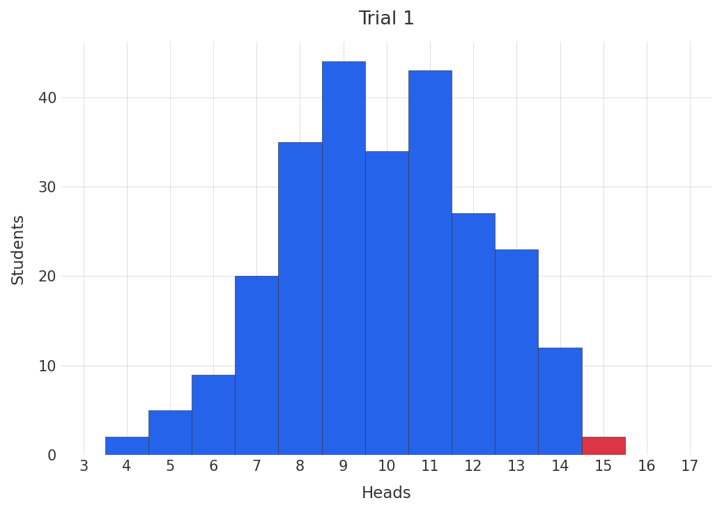
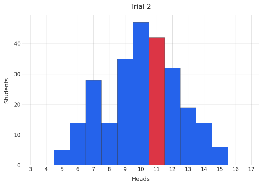
This time, we have strong reason to expect (and confirmed in the plot below, original winner shown in red) that the best performers from the last tournament would not perform as well in this tournament ². Their relatively extreme performance during the first tournament will regress toward the mean performance.

Putting them to the Test

To consider a different example, let’s now imagine administering a test to our school of 256 students. The test has been designed to be fairly hard, with the average student having only a 50% chance to get a given question correct and ~95% of the students having between a 30% and a 70% chance of getting a given question correct ³. Due to the cost of grading the test, the number of questions have been kept at 20.

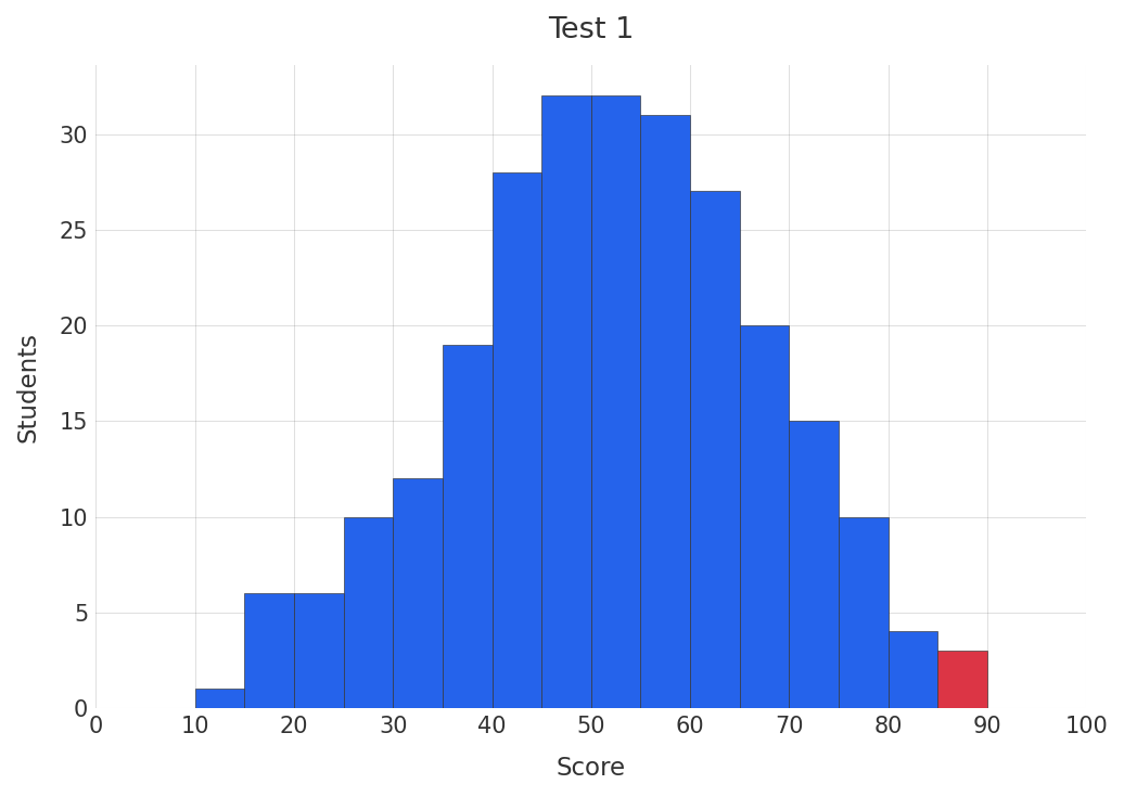
The above graph shows a simulated grade distribution for the above scenario, with the bin containing the best performing student highlighted in red.

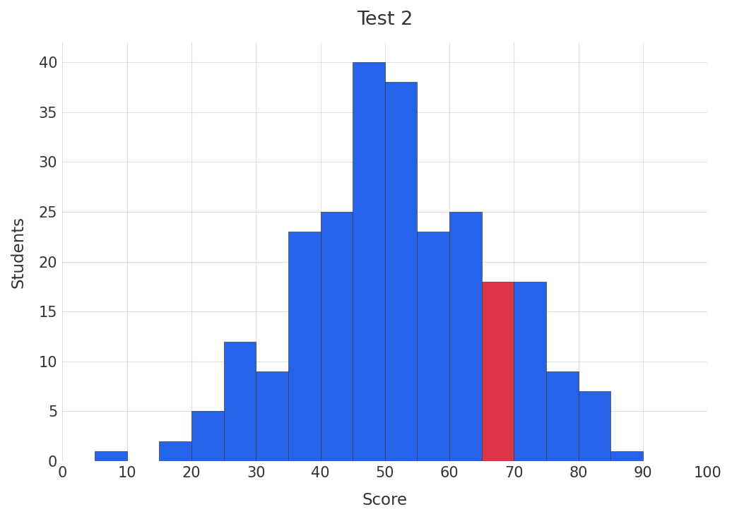
Now, let’s imagine we adminster a similar test again. How does our best student perform? Once again, the simulated grade distribution is plotted above with the bin containing that student in red. Notably, the student performs worse on the second test. Once again, we notice regression toward the mean, although the effect is more modest.

Luck and Skill

The simplest way to understand regression toward the mean (although this doesn’t describe regression toward the mean in a fully general fashion) is that performance is described by two components: luck and skill. In some domains, luck dominates. In other domains, skill dominates.

When you observe someone’s performance over the short run, their performance may be dominated by outlier values (both higher or lower than their long run performance). With repeated sampling, variability (under many circumstances) cancels out, giving you a reasonable estimate of the individual’s skill.

Regression toward the mean can also be applied at the population level (such as in both of the above cases). In these cases, one has both individual level variability (some individuals are more skilled than other individuals) and population level variability (due to the population skill distribution). A priori, we should expect individuals to tend to regress toward the mean of the population, with the effect more pronounced for larger populations (as there are more chances for a significant outlier to occur).

New Recipes and Becoming a Better Cook

It’s Sunday afternoon, you have some spare time, and decide to find a new recipe to cook. You search online, find a new recipe, cook it, and are shocked at how good it is. It’s so good, in fact, that you resolve to cook it tomorrow night. The next time you cook it, however, it fails to live up to your expectation - why? Is this another case of regression toward the mean?

To explore a more explicit model of why regression toward the mean occurs, let’s decompose what might be some of the determinants of a recipe’s success:

1. The recipe
2. Ingredient freshness
3. Cooking skill

What has changed between today and yesterday? Well, the recipe is the same, but perhaps you mismeasured some of the ingredients today (or yesterday). The freshness of ingredients decays with time, and the ingredients used today may be at varying degrees of freshness (with varying degree of impact on recipe output). Finally, perhaps you are either executed the recipe better (or worse) today. The key point, however, is that the recipe’s “goodness” is a function of many factors and these are changing randomly (well, relative to you). Your decision to cook the recipe again, however, is non-random. It’s largely because the recipe was an outlier. This gives rise to regression toward the mean.

With that in mind, the above model allows one to recognize the key generators of cooking skill (at least within the context of this example, real cooks please forgive me). A better cook develops better recipes, selects better ingredients, and is more effective at executing on the recipe. Initially, much of the “luck” in whether a recipe is good is simply epistemic uncertainty about what makes a recipe good.

Don’t Jinx It

It’s approaching the end of January and you’ve had a surprisingly mild winter. One might feel tempted to utter the words “this winter has been surprisingly mild”, but this temptation is blunted by a (rather irrational) fear that by simply uttering the words “mild winter” you will call upon Jack Frost to descend upon the world, turning it into a winter wasteland. Surprisingly, this might also be best considered an example of regression toward the mean.

As a simple example, imagine there is a 20% chance of a winter storm on a given winter day. On the vast majority of winter days, there will be no snowfall. The average number of days between snowfalls might be three (or so), but the average hides a surprising amount of variation. It’s not too uncommon, for example, for one to observe a ten day streak without snow. Upon observing such a hot streak, however, the odds that the hot streak continues for the same duration is vanishingly small. At some point, the luck runs out and one observes a winter storm. You didn’t jinx it, your luck simply ran out.

From the perspective of a statistically ignorant observer, one feels like the noticing of a surprising streak inevitably coincides with the end to that surprising streak. This, however, is an illusion. The odds of the streak ending are relatively constant across time, what varies is your surprise at observing the state. The longer the streak, the more one feels like the observation of the streak ultimately causes it’s end ⁴.

The Placebo Effect

The same intuition underpinning our willingness to believe in jinxes may also (partially) explain the placebo effect.

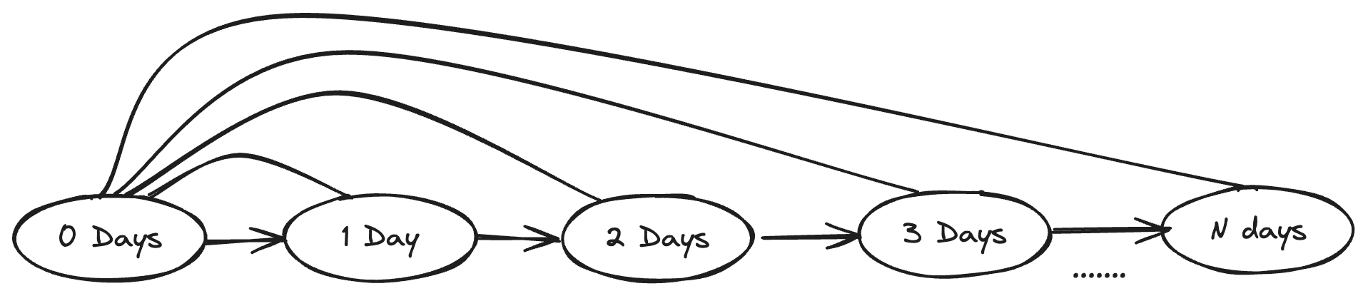
To consider just a simple model, let’s imagine that the likelihood you visit a doctor is described by a simple function:

1. Have you been sick for at least three days?
2. If you’ve been sick for three days, the likelihood you visit the doctor increases with every passing day.

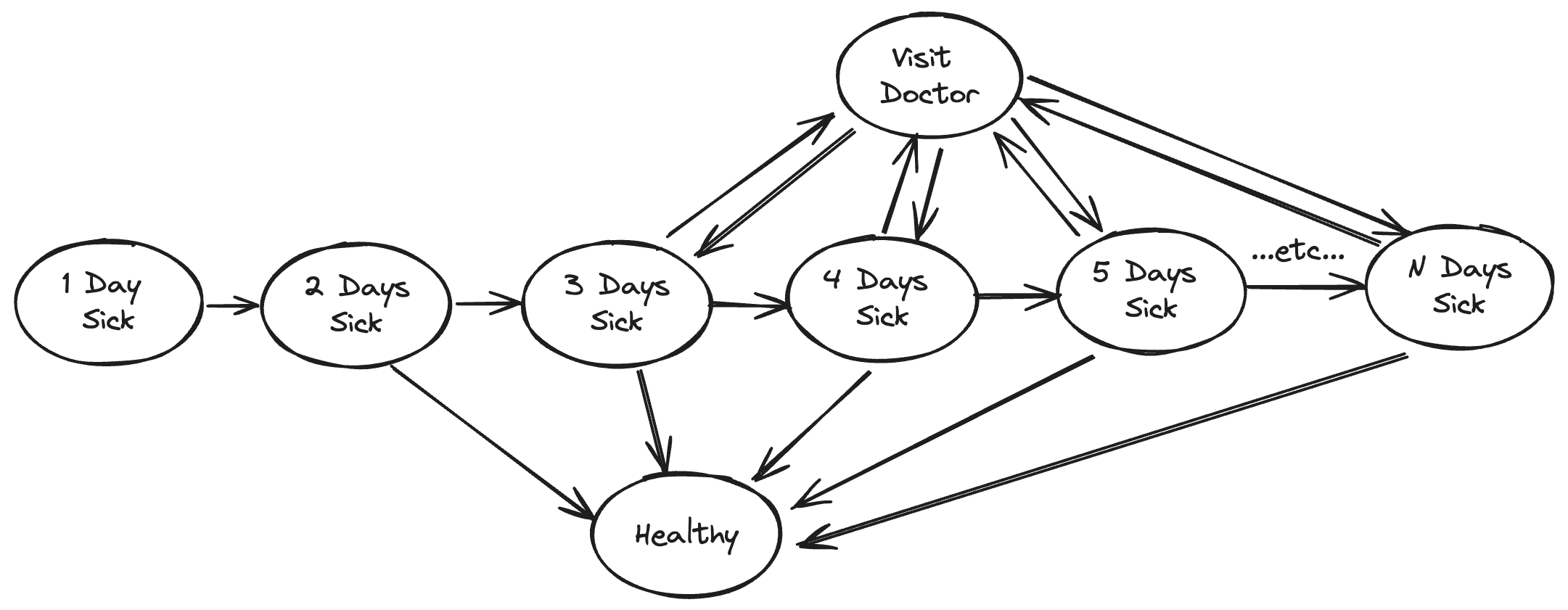
In addition, let’s posit that the likelihood of your recovery is also a function of how long you have been sick.

Under such a simple model, one observes a correlation between “visiting the doctor” and “days until recovery”. This correlation, however, is largely a selection artifact. The relationship between “visiting the doctor” and “days until recovery” exists because individuals feel compelled to visit the doctor after being sick for a period of time. In different terms, individuals tend to visit the doctor when they are at their sickest and, unless the disease is life threatening, that is the point at which they are most likely to being to recover. Once again, the individual regresses toward the mean.

Why Care?

Regression toward the mean applies to any situation in which short-run performance is dominated by non-repeatable variation. In domains with significant degrees of non-repeatable variation, outliers will tend to be outliers due to that variation, not due to whatever factors are responsible for their long-run performance.

The most practical reason to care about regression toward the mean is the remarkable ease with which one can fool oneself into mistaking statistical artifacts for genuine results. That new feature you launched to try and get out of a slump? You would have gotten out of the slump anyways. That new heralded machine learning model that you trained and deployed to production? You wouldn’t be excited about it if it didn’t perform well, but it’s performance should lead one to be suspicious about it’s long run performance. That supposedly promising new hire who failed to execute to your expectations on their first project? Perhaps they simply were unlucky, best to temper your pessimism.

Organisationally, combatting regression towards the mean requires one measure performance, account for the natural variability in performance, and adjust for population size. Ensure that what you are measuring is what you are interested in and that it continues to remain what you are interested in across time. Recognize that the short-run is not always indiciative of the long-run, and what constitutes short-run and long-run is domain dependent. Remember the wildly improbably happens every day if your population is large enough.